Introduction
Here is presented how to use all TnetRUI and T-NET code in order to study the impact of ripysylve vegetation on river temperature.
exempleData <- TNETutils_openExempleData()
segments <- st_read(exempleData$Shapefile_segments,quiet = TRUE)
nodes <- st_read(exempleData$Shapefile_nodes,quiet = TRUE)Pre work
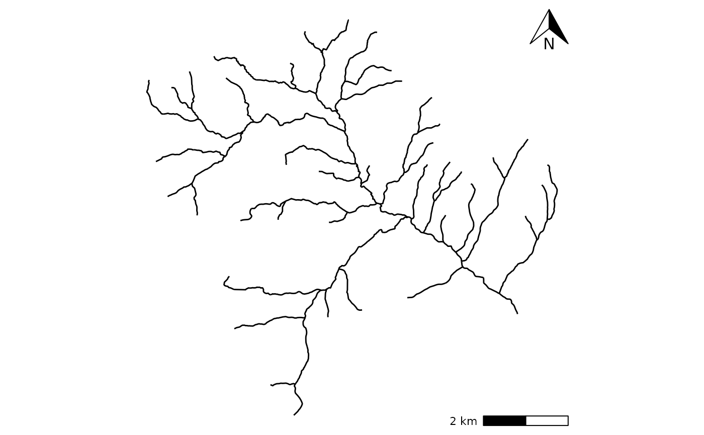
All TnetRUI function will be based on TOPAGE river data
Before using TnetRUI functions, some work needs to be done on the river network.
Cleaning the network
First, some cleaning on the TOPAGE raw river network needs to be done:
Removing all not-natural segments
Removing all segments not connected to the principal river network
Deleting loops in the river network
Cleaning triple confluences when possible
In the future, it will be possible to do these work inside of TnetRUI.
Adding J2000/EROS coupling
Each segments in the network needs to be linked to a J2000 or EROS segment in order to get Disharge from them
This needs to be done manually, nothing will be added in the futur in TnetRUI in order to do that.
Each segments needs to have the following info in the result shapefile:
| Columns Name | Descrition |
|---|---|
| J2000 | ID of the J2000 segments |
| P_J2000 | 1 if the segment is the most downstream segments linked to the J2000 ID, 0 if it’s not |
Adding vegetation info
Each segments in the network needs to have information on the ripysilve vegetation
Each segments needs to have the following info in the result shapefile:
| Columns Name | Descrition |
|---|---|
| RG_PCT_VEG | Percentage of river left bank covered by vegetation (0 - 100) |
| RG_H_MOY | Mean height of the vegetation on the left bank |
| RD_PCT_VEG | Percentage of river right bank covered by vegetation (0 - 100) |
| RD_H_MOY | Mean height of the vegetation on the right bank |
Checking the shapefile
Before running functions in the TnetRUI package, it is possible to
use TNETutils_checkShapefile() to verify if all the needed
columns are present in the shapefile and if the missing ones are
computable with function in the TnetRUI package.
TNETutils_checkShapefile(segments,hydro_model = 'J2000')
#> ══ Columns needed to use TNET and TNETshape functions with the hydrological mode
#> ── 21 columns needs to be computed ─────────────────────────────────────────────
#> 18 columns are needed for TnetRUI functions.
#>
#> ! 16 computed by `TnetRUI::TNETshape_getSafran()`
#> ID_M_1, ID_M_2, ID_M_3, ID_M_4, ID_M_5, ID_M_6, ID_M_7, ID_M_8, Rap_M_1, Rap_M_2, Rap_M_3, Rap_M_4, Rap_M_5, Rap_M_6, Rap_M_7, Rap_M_8
#> ! 2 computed by `TnetRUI::TNETshape_computeCoefQcalc()`
#> RppAr_v, RppA_BV
#> 3 columns not needed for TnetRUI but for T-NET model.
#>
#> ! 3 computed by `TnetRUI::TNETshape_computePosition()`
#> Xcentr, Ycentr, phi_deg
#> ── 10 columns are present ──────────────────────────────────────────────────────
#> gid_new, ID_ND_INI, ID_ND_FIN, RG_PCT_VEG, RD_PCT_VEG, RG_H_MOY, RD_H_MOY, Longueur_m, J2000, P_J2000
#> ℹ More info about missing columns can be found in the documentation on TnetRUI website (<https://tnet-rui-guillaume-hevin-ff27f1d42adcce7ceedbb780ef0d88b292c862.pages.mia.inra.fr/articles/TnetRUI.html>)
#> ════════════════════════════════════════════════════════════════════════════════We can see that columns needs to be computed by
TNETshape function. This is what will by creating the river
network.
Create the river network
One’s you have done the previous steps, your are ready to run all TNETshape functions in order to compute whats needed for TNET to work. All the informations needed are the following:
Drain area
SAFRAN grid IDs
Position
Orientation
J2000 coeficients
All of these steps are detailed in the article “1. How to use TNETshape functions” and can be launch using
TNETshape_prepare().
Drain area
The computation of drain area is made by
TNETshape_computeAreaDrain() and use Whitebox to do all of the
computations (Whitebox needs specifique installation steps that can be
found here). This function permite to compute
both total drain area and sub-watershed drain
area which is the drain area of the segment only (show on the
figure bellow)
#We want to set manually the upstream moving distance of the exutoire
ID_spe <- data.frame(gid_new = 1615891,
Recul = 85)
#compute Drain area
shape_drainArea <- "test/1_DrainArea_Ardiere.shp"
TNETshape_computeAreaDrain(path_DEM = exempleData$DEM,
path_segments = exempleData$Shapefile_segments,
path_node = exempleData$Shapefile_nodes,
export_file = shape_drainArea,
ID_special = ID_spe)
#> Moving segments nodes ■■■■■■■■ 22% | ETA: 4s
#> Moving segments nodes ■■■■■■■■■■■■■■■■■■■■■■■ 72% | ETA: 1s
#> Moving segments nodes ■■■■■■■■■■■■■■■■■■■■■■■■■■■■■■■ 100% | ETA: 0s
#> Problems on drain area calculations was found on 2 segments:
#> 2 segments have a drainage area exceeding 40% of their upstream segment. (Threshold_limit)
#> All affected segments are saved in Area_problem.shp shapefile.SAFRAN grid ID
Now we want to extract in which SAFRAN grid each segments is in. For
that, we can use the function TNETshape_getSafran()
function as following: Each segments can be at maximum in 8
SAFRAN grid at the same time
#compute Drain area
shape_SafranID <- "test/2_SafranID_Ardiere.shp"
TNETshape_getSafran(path_segments = shape_drainArea, #We use the shape made before
path_SafranGRID = exempleData$SAFRAN_grid,
export_file = shape_SafranID)Segments Position and orientation
Both Segments positions and orientation are calculated with the
function TNETshape_computePosition().
Position is defined as the middle of the line between the initial and final node (in WGS84).
Orientation as the angle between North and the oriented line between the initial and final node.
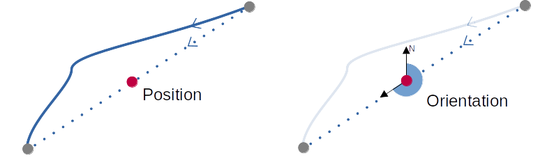 It’s calculated the following way:
#compute Drain area
shape_Position <- "test/3_Position_Ardiere.shp"
TNETshape_computePosition(path_segments = shape_SafranID, #We use the shape made before
path_nodes = exempleData$Shapefile_nodes,
export_file = shape_Position)J2000 coeficients
All J2000 coeficients are computed with the function
TNETshape_computeCoefQcal().
this is how it is omputed:
#compute Drain area
shape_Qcoef<- "test/4_Qcoef_Ardiere.shp"
TNETshape_computeCoefQcalc(path_segments = shape_Position, #We use the shape made before
export_file = shape_Qcoef)Now everything is setup in order to prepare and run an TNET
modelisation
Prepare data for T-NET
This will used all TNET set function in order to create all data
needed by TNET.
Initialize the simulation
It’s possible to create a pre-filled main file using
tnet_create_main()function.
It is better at the beginning to use the
TNET_initializeSim() in order to regroup all needed
parameters for all functions. All arguments used here are set for the
example data in the shapefile
infoSimu <- TNET_initializeSim(name_simu = 'TNET_Ardiere',
year_start = 2017,
year_end = 2021,
weather_model = 'SAFRAN',
hydro_model = 'J2000',
path_J2KResult = exempleData$J2K_path,
path_J2Kparameter = exempleData$J2K_path,
path_Export = 'test',
shapefile = shape_Qcoef,
path_safran_inputNetCDF = exempleData$SAFRAN_path,# "file.path("/home/ghevin/Documents/T-NET/Code/TnetRUI/","inst","extdata","Safran"),
path_TNET = '/home/ghevin/Documents/T-NET/Code/TNET/sources')
# # #Preparing all data
All needed data can be prepared with the function
TNET_prepareSim() and the infoSimu variable
created before
# Deprecated
# TNET_prepareSim(infoSimu,prepare_meteo = FALSE,export_Qb = TRUE)
#Reading SAFRAN files
tnet_safran_readfiles(folder_data = infoSimu$path_safran_inputNetCDF,
folder_export = infoSimu$path_safran,
shapefile = infoSimu$shapefile,
date_start = infoSimu$start_simu,
date_end = infoSimu$end_simu,
source = "INRAEpnas")
#> ⠙ Reading SAFRAN Data: Preparing computation
#> ⠹ Reading SAFRAN Data: Reading NetCDF data files [1/5]
#> ⠸ Reading SAFRAN Data: Reading NetCDF data files [2/5]
#> ⠼ Reading SAFRAN Data: Reading NetCDF data files [3/5]
#> ⠴ Reading SAFRAN Data: Reading NetCDF data files [4/5]
#> ⠦ Reading SAFRAN Data: Reading NetCDF data files [5/5]
#> ✔ Finished reading SAFRAN Data [54.6s]
#>
#Reading J2000 files
TnetJ2K_readfiles(path_J2Kfile = infoSimu$path_J2KResult,
path_Export= infoSimu$path_tmp,
date_start = infoSimu$start_simu,
date_end = infoSimu$end_simu,
path_J2Kpar = infoSimu$path_J2Kparameter)
#> ⠙ Reading ReachLoop.dat file from J2000 simulations: Preparing computations
#> ✔ Reading ReachLoop.dat done ! [1.1s]
#>
#> ⠙ Reading HRULoop.dat file from J2000 simulations: Preparing computations
#> ⠹ Reading HRULoop.dat file from J2000 simulations: 99%
#> ✔ Reading HRULoop.dat done ! [913ms]
#>
#Computing discharge on T-NET network
TnetJ2K_computeQ(path_data = infoSimu$path_tmp,
path_export = infoSimu$path_hydro,
shapefile = infoSimu$shapefile)
#> ⠙ Computing discharge data (Q): Preparing computations
#> ✔ Computing discharge (Q) done ! [605ms]
#>
#Computing hydraulic data
TnetHydraulic_width(path_data = infoSimu$path_hydro,
shapefile = infoSimu$shapefile,
method = 'Morel')
#> ⠙ Computing river width: Preparing computations
#> ✔ Computing river width done ! [247ms]
#>
TnetHydraulic_depth(path_data = infoSimu$path_hydro,
shapefile = infoSimu$shapefile,
method = 'Morel')
#> ⠙ Computing river depth: Preparing computations
#> ✔ Computing river depth done ! [252ms]
#>
TnetHydraulic_travelTime(path_data = infoSimu$path_hydro,
shapefile = infoSimu$shapefile)
#> ⠙ Computing river travel time: Preparing computations
#> ✔ Computing river travel time done ! [260ms]
#>
#> ℹ Some water travel time where found <1h on 121 segments (100%). This can produce instabilities on water temperature modelisation
#Computing underground lateral discharge
TnetJ2K_computeQlatSout(path_data = infoSimu$path_tmp,
path_export = infoSimu$path_hydro,
shapefile = infoSimu$shapefile,
path_J2K_reachpar = infoSimu$path_J2Kparameter,
export_Qb = TRUE)
#> ⠙ Computing underground discharge (Qlat_ms): Preparing computations
#> ⠹ Computing underground discharge (Qlat_ms): 100%
#> ✔ Computing underground discharge (Qlat_ms) done ! [1s]
#>
#Computing underground water temperature
TnetJ2K_computeTg(path_data = infoSimu$path_safran,
path_export = infoSimu$path_hydro,
shapefile = infoSimu$shapefile)
#> ⠙ Computing undergroud temperature (Tg): Preparing computations
#> ✔ Computing undergroud temperature (Tg) done ! [648ms]
#>
TNET_createShape(shapefile = infoSimu$shapefile,
shapefileExport = infoSimu$name_shape,
columns_toKeep = NULL ) # Can be any column to keep in the shapefile (ex: c("TopoOH","OSTRAHLER"))Running simulation
The simulation is run with the following function
TNET_run()
TNET_run(infoSimu,
Name = "Simulation_Normal",
variableExport = c("SF","Tw_NFS"))
#> ❯ Execution de T-NET: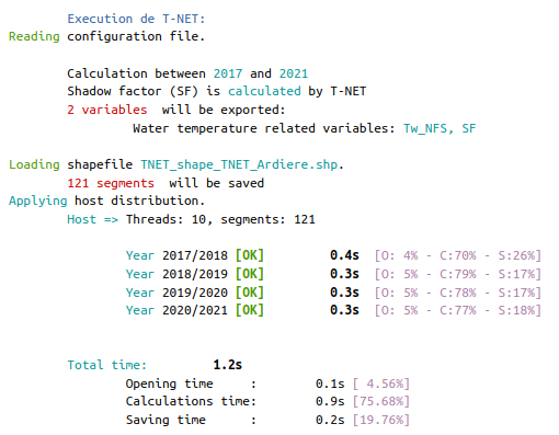
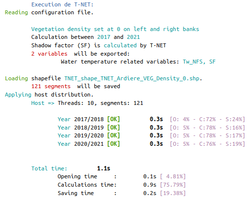
Study case: How does the water temperature change with the amount of rypisilve vegetation
In this case scenatio we will take the results of the simulations made before and compare them with a new simulation where all vegetation on the watershed was set to 0
The code to run the new simulation is the following:
infoSimu$name_shape <- TNETveget_modify(infoSimu$name_shape,density = 0)
TNET_run(infoSimu,
Name = "Simulation_Veg_0",
variableExport = c("SF","Tw_NFS"))
#> ❯ Execution de T-NET:
#
Plot both results
Here we can plot both result at the most downstream segments:
result_normal <- file.path('test','TNET_Ardiere','results','Simulation_Normal','Tw_NFS.nc')
result_veg0 <- file.path('test','TNET_Ardiere','results','Simulation_Veg_0','Tw_NFS.nc')
downstream_ID = 1615891
dayStart <- "2018-01-01"
dayEnd <- "2018-12-31"
#Reading results fom files
data_normal <- TNETresult_read(result_normal,
date_start = dayStart,
date_end = dayEnd,
ID = downstream_ID,
format_long = TRUE)
data_veg0 <- TNETresult_read(result_veg0,
date_start = dayStart,
date_end = dayEnd,
ID = downstream_ID,
format_long = TRUE)
#Combine both results
data_normal$Scenario <- 'Normal'
data_veg0$Scenario <- "Vegetation = 0%"
data <- rbind(data_normal,data_veg0)
#Compute daily results
data$day <- text_toDate(format(as.POSIXct(data$Date), "%Y-%m-%d"))
data_day <- data[,.(Tw_NFS = mean(Tw_NFS)),by=c('Scenario','gid','day')]
data_day$Date <- data_day$day +hours(12)
##Prepare Plot
data_day$H <- 'Daily results'
data$H <- 'Hourly results'
data <- rbind(data,data_day)
data$Scenario <- factor(data$Scenario,levels = c("Vegetation = 0%",'Normal'))
data$H <- factor(data$H,levels = c('Hourly results','Daily results'))
plt <- ggplot(data, aes(x=Date,y=Tw_NFS,color = Scenario))+
geom_line()+
labs(y = "Water temperature (°C)")+
theme_bw()+
facet_wrap(c('H'),ncol = 1,scales = "fixed")
ggplotly(plt, dynamicTicks = TRUE)Compare both simulations
Lets compare how cutting simulations will impact the mean temperature during a hot summer day, for example 2018-08-01
library(viridis)
day <- "2018-08-01"
Compare <- TNETresult_compare(NetCDF_reference = result_normal,
NetCDF_toCompare = result_veg0,
date = day,
column_keep = c( "vegPctL", "vegPctR"))
## Plot Temperature diff
plt <- ggplot(data = Compare)+
geom_sf(aes(geometry =geometry, color = diff))+
scale_color_viridis(option = "C")+
theme_void()+
labs(color = "",
title = paste("T° difference between Normal and 0 vegetation (",day,")"))
ggplotly(plt)
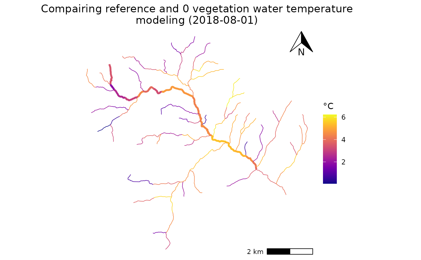
## Plot Temperature diff
library(ggspatial)
ggplot(data = Compare)+
geom_sf(aes(geometry =geometry, color = data_ref))+
annotation_scale(plot_unit = "m",location = 'br')+
annotation_north_arrow(location = 'tr',width = unit(1,'cm'),height = unit(1, "cm"))+
scale_color_gradient2(low = "#2d7ab6",
high = "#d6191c",
mid = "#feffbe",
# Make the gradient2 "switch" at a midpoint of 13
midpoint = 19)+ #low = ,mid="#feffbe",high = "#d6191c"
theme_void()+
labs(color = "°C",
title = paste0("Water temperature (",day,")"))+
theme(plot.title = element_text(hjust = 0.5))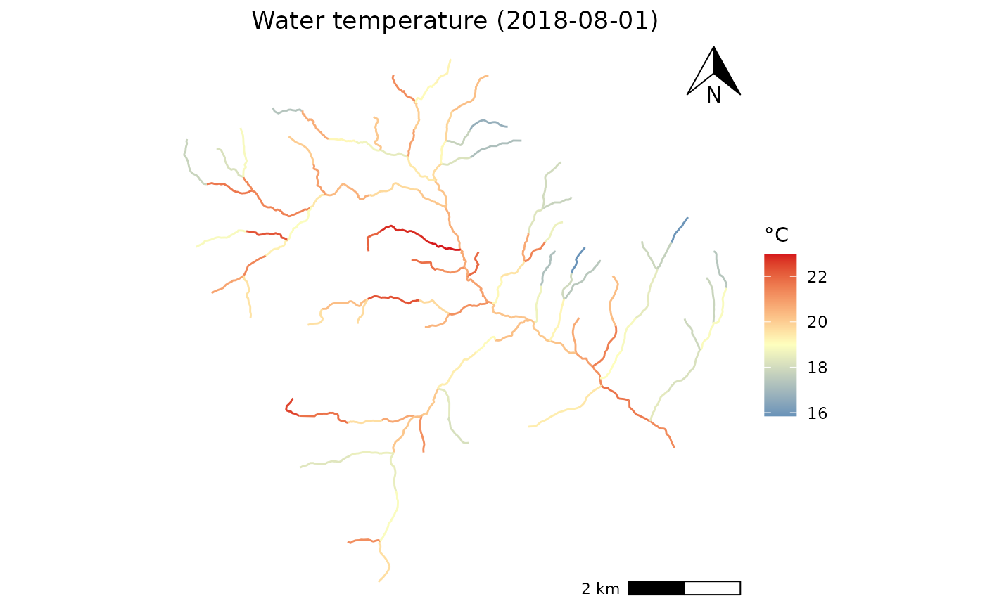
ggplot(data = Compare)+
geom_sf(aes(geometry =geometry, color = diff))+
annotation_scale(plot_unit = "m",location = 'br')+
annotation_north_arrow(location = 'tr',width = unit(1,'cm'),height = unit(1, "cm"))+
scale_color_viridis(option = "C")+
theme_void()+
labs(color = "°C",
title = paste0("T° difference between Normal and 0 vegetation (",day,")"))+
theme(plot.title = element_text(hjust = 0.5))
#Compute mean vegetation difference
Compare$VegMoy_diff <- (Compare$vegPctL_diff + Compare$vegPctR_diff)/2
## Plot Vegetation diff
plt <- ggplot(data = Compare)+
geom_sf(aes(geometry =geometry, color = VegMoy_diff))+
scale_color_viridis(option = "D")+
theme_void()+
labs(color = "",
title = paste("Vegetation difference between Normal and 0 vegetation (",day,")"))
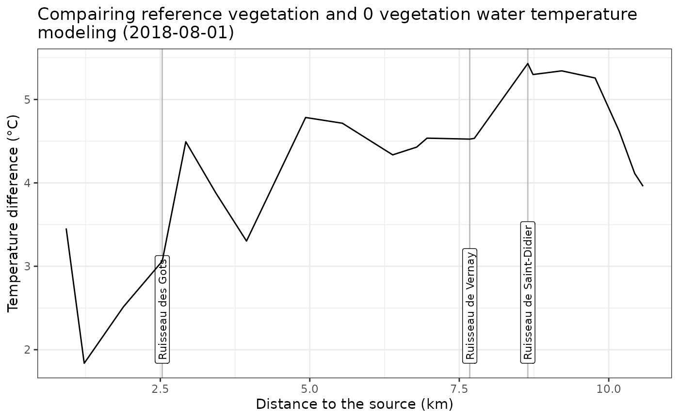
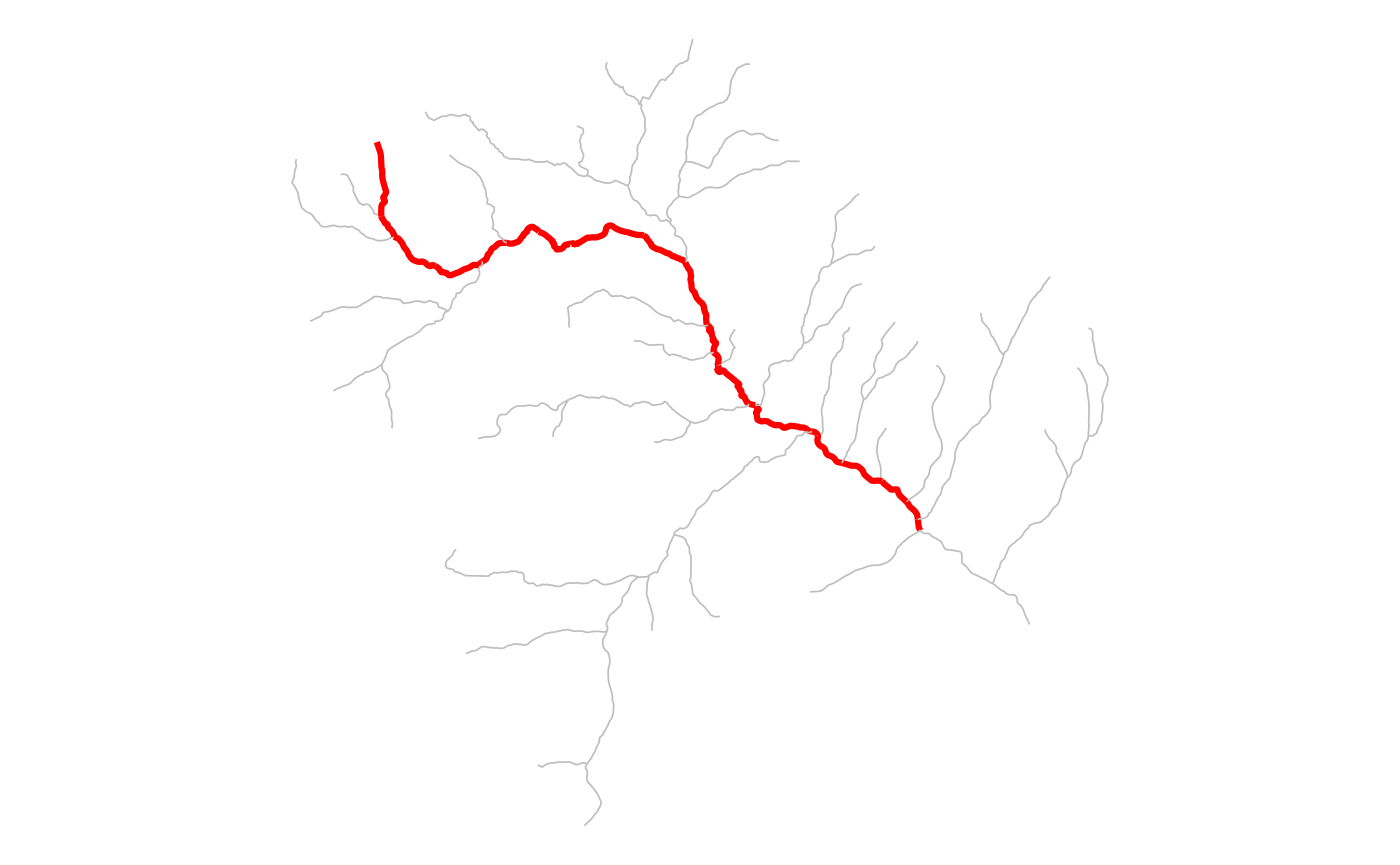
ggplotly(plt)Compare both simulation with a Longitudinal profile
It’s also possible to compare the data using a longitudinal profile
plot on the main chanel using
TNETutils_getLongProfile():
GID_START_plot = 2049842
GID_END_plot = 1760774
confluence_toPlot <- data.frame(ID = c(2687405,2860857,2684740),
name = c('Ruisseau de Saint-Didier','Ruisseau de Vernay','Ruisseau des Gots'))
long_compare <- TNETutils_getLongProfile(troncons = Compare,
ID_ini = GID_START_plot,
ID_fin = GID_END_plot,
columns_keep = c('data_ref','data_cmp','diff'),
confluence_toAdd = confluence_toPlot$ID)
confluences <- TNETutils_getLongProfileConfluence(long_compare,y='diff')
confluences <- merge(confluences,confluence_toPlot,by.x="LABEL",by.y = "ID")
plt <- ggplot(data = long_compare, aes(x=L_Upstream,y=diff))+
geom_vline(xintercept = confluences$X, color = 'grey')+
geom_label(data = confluences,aes(x=X, y=Y, label=name), angle=90,hjust = 0,fill='white',size = 3)+
geom_line()+
theme_bw()+
labs(x="Distance to the source (km)",
y = 'Temperature difference (°C)',
title = paste0("Compairing reference vegetation and 0 vegetation water temperature\nmodeling (",day,")"))
print(plt)